|
|
||||
|
|
|
|
|
|
Starting Lesson for Excel
This lesson will teach you about relative cell addresses, how to enter data into cells, how to enter formulas into cells, copying and pasting cell contents, and will introduce you to functions and the Data Analysis tool. It will then describe the naming convention for the remaining files in this folder. All the following lessons assume you have completed this lesson first. It is best to print each lesson and work from a hard copy. Each lesson assumes you are sitting in front of your computer with a blank Excel spreadsheet open.
Relative Cell Addresses
The major part of an Excel worksheet consists of a grid with columns labeled A, B, C and so on, and rows labeled 1, 2, 3, and so forth.
|
A |
B |
C |
D |
|
|
1 |
||||
|
2 |
||||
|
3 |
||||
|
4 |
Each of the rectangles (cells) inside the grid is named by the column and row it is in. For example, the cell with the "C3" written in it is actually named C3 because it is in Column C and it is in Row 3. The cells address is C3.
|
A |
B |
C |
D |
|
|
1 |
||||
|
2 |
||||
|
3 |
C3 |
|||
|
4 |
The white rectangle above A is the name box which shows the name of the cell (usually the same as the address unless you give it another name). The white rectangle above C, D, E is the formula bar.
|
C3 |
= |
|||
|
A |
B |
C |
D |
|
|
1 |
||||
|
2 |
||||
|
3 |
| |
|||
|
4 |
||||
If you were to type the number 45 in cell C3 the number would also appear in the formula bar and the number 45 would be on the left side of the cell.
|
C3 |
X / = |
45 |
||
|
A |
B |
C |
D |
|
|
1 |
||||
|
2 |
||||
|
3 |
45| |
|||
|
4 |
||||
(In the cell above "B," I am using a / to represent a check mark - this way I don't need to use a special character.)
Once you press return, the number 45 will jump to the right side of the cell (an entry containing letters would have staid on the left) and your cursor would move to another cell (the one to its right "D3" or the one below it "C4" depending on how your options are set). Hitting enter, enters the number in the cell.
|
C3 |
X / = |
45 |
||
|
A |
B |
C |
D |
|
|
1 |
||||
|
2 |
||||
|
3 |
45 |
| |
||
|
4 |
||||
Next enter 67 in cell C4.
|
C3 |
X / = |
45 |
||
|
A |
B |
C |
D |
|
|
1 |
||||
|
2 |
||||
|
3 |
45 |
|||
|
4 |
67 |
| |
||
Relative Cell Addresses / Formulas
Now we will learn how to enter a formula. Put your cursor in D3 (the cell to the right of C3). Type the equal sign (=). The equal sign lets the program know that you will be entering a formula. Then type C3+2
|
C3 |
X / = |
=C3+2 |
||
|
A |
B |
C |
D |
|
|
1 |
||||
|
2 |
||||
|
3 |
45 |
=C3+2| |
||
|
4 |
67 |
|||
When you press enter, the number 47 will appear in cell D3. You would think that this is because you instructed your computer to add what ever was in cell C3 and 2. Since the value in C3 is 45, the program adds 45 + 2 and gets 47.
|
D4 |
X / = |
=C3+2 |
||
|
A |
B |
C |
D |
|
|
1 |
||||
|
2 |
||||
|
3 |
45 |
47 |
||
|
4 |
67 |
| |
||
But, that is not exactly the way the program works. Excel is, by default, a relational spreadsheet program. This relational aspect may seem strange at first, but it is what gives Excel so much power. When you typed in =C3+2, you told the program to take the value in the cell one to the left and add 2 to it. Don't believe me? Let's check it out. Click on D3 and then copy (I do this by pressing Ctrl + c that is, I hold the control button down as I press c). (If you are more used to copying by selecting Edit then copy, please feel free to do it that way.) Wow, isn't that weird. When you copy a cell, a bunch of ants march around that cell - around and around.
Now we will paste this material in cell D4. I do this by pressing Ctrl + v, but you can use Edit paste, if you would rather.
|
D4 |
= |
=C4+2 |
||
|
A |
B |
C |
D |
|
|
1 |
||||
|
2 |
||||
|
3 |
45 |
47 |
||
|
4 |
67 |
69 |
||
What is this? It says 69 not 47. And, the formula bar - it says =C4+2. That is because the formula really said, take the value of the cell to the left of this cell and add 2 to it. What value do you think would appear if we pasted our formula into E3? What value would appear if we paste into B2? What value would appear if we were to paste our formula into A3? The answers are 49 (47 + 2), 2 (blank +2) and #NUM (there is no cell to the left of A3 so we get an error).
Ok Ok Ok - As long as we are getting weird, let's try something really wild. Click in cell E3 then type the equal sign (But do not press Enter).
|
E3 |
X / = |
= |
|||
|
A |
B |
C |
D |
E |
|
|
1 |
|||||
|
2 |
|||||
|
3 |
45 |
47 |
= |
||
|
4 |
67 |
69 |
|||
Now click on cell C3,
|
E3 |
X / = |
=C3 |
|||
|
A |
B |
C |
D |
E |
|
|
1 |
|||||
|
2 |
|||||
|
3 |
45 |
47 |
=C3 |
||
|
4 |
67 |
69 |
|||
"C3" now appears in both the formula bar and in cell E3 and ants march around cell C3. Now, press the asterisk (which is shift + 8 and means multiply) then 2 and enter.
|
E4 |
X / = |
=C3 |
|||
|
A |
B |
C |
D |
E |
|
|
1 |
|||||
|
2 |
|||||
|
3 |
45 |
47 |
90 |
||
|
4 |
67 |
69 |
| |
||
The moral of this is that there are two ways of entering cell addresses into your formula, you can type them in or you can just click on the cell and the address will be put in the formula automatically.
Now let's clear the spreadsheet so we can try some other tricks. There is a gray cell that is just to the left of the A and just above the 1. Click on that cell and all the cells but A1 will become black.
|
|
A1 |
= |
|||
|
A |
B |
C |
D |
E |
|
|
1 |
|||||
|
2 |
|||||
|
3 |
45 |
47 |
90 |
||
|
4 |
67 |
69 |
| |
||
Then press your delete key, and all the numbers you entered earlier will disappear. Click on A1. Now enter the following numbers until your spreadsheet looks like the one below.
|
= |
|||||
|
A |
B |
C |
D |
E |
|
|
1 |
1 |
2 |
3 |
||
|
2 |
4 |
5 |
6 |
||
|
3 |
7 |
8 |
9 |
||
|
4 |
10 |
11 |
12 |
| |
|
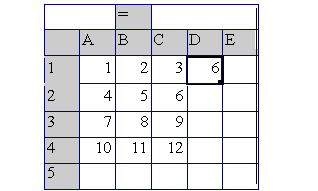
Now go to cell D1. Enter the formula = A1+B1+C1 Enter. Then click back on cell D1.

This gives you the sum of the numbers in the first row. See the dark outline around cell D1? See the little black square (exaggerated in the picture above) at the lower right corner of that cell? The little square in the corner is called the "handle."
Without pressing the mouse button, move your cursor around the spreadsheet. You will notice that the cursor is a wide plus sign. However, if you move the cursor (still without pressing the mouse button) onto the handle, it becomes a thin plus sign. Don't you wish you could lose weight that fast?
Move the cursor over the handle until you get the thin plus sign, then while the cursor is thin, press and hold the left mouse button down. While holding down the mouse button, move the cursor down until it captures cells, D1, D2, D3, and D4 then let go of the mouse button.
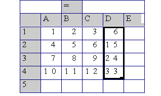
Once you have put in the formula for the first row, see how easy it is to get the spreadsheet to calculate the sum of the remaining rows? If you click on cell D1, you will see the formula you entered (=A1+B1+C1). If you click on cell D2, you will see =A2+B2+C2. If you click on cell D3, you will see =A3+B3+C3. If you click on cell D4, you will see =A4+B4+C4.
Functions
Entering =A1+B1+C1 was a little bit time consuming. Just imagine if we had 30 rows of data typing in =A1+B1+C1+D1+E1+F1+G1+H1+I1+J1+K1+L1+M1+N1+O1+P1+Q1 . . .AB1+AC1+AD1. What a drag!!! Fortunately, we can use functions and cell ranges instead. Let's try using functions and cell ranges to sum up the columns of numbers on our spreadsheet. First, put your cursor in cell A5. We are going to find an easier way to enter the equivalent of "=A1+A2+A3+A4." Instead type "=SUM(A1:A4)" then press enter.
|
A6 |
= |
||||
|
A |
B |
C |
D |
E |
|
|
1 |
1 |
2 |
3 |
6 |
|
|
2 |
4 |
5 |
6 |
15 |
|
|
3 |
7 |
8 |
9 |
24 |
|
|
4 |
10 |
11 |
12 |
33 |
|
|
5 |
22 |
||||
|
6 |
|||||
Let's break down what you typed into its parts. The "=" tells the program you are entering a formula. The "SUM( )" tells the program that you want it to run the sum function. And, the "A1:A4" tells your program to apply the function to the block of cells starting with A1 as the top left cell and going to A4 as the bottom right cell.
Now click on cell A5, grab its handle and pull it to the right (not down) to include columns B, C, and D. Remember how to pull its handle? If not, please review the material above.
|
D6 |
= |
||||
|
A |
B |
C |
D |
E |
|
|
1 |
1 |
2 |
3 |
6 |
|
|
2 |
4 |
5 |
6 |
15 |
|
|
3 |
7 |
8 |
9 |
24 |
|
|
4 |
10 |
11 |
12 |
33 |
|
|
5 |
22 |
26 |
30 |
78 |
|
|
6 |
|||||
Now, let's think about what we have. Cells A1:C4 contains our original data. Cells D1:D4 contain the row columns. Cells A5:D5 contain the column totals. Cell D5 is the sum of all the row totals - it is, therefore, also the total sum of all our original data.
|
D6 |
= |
||||
|
A |
B |
C |
D |
E |
|
|
1 |
1 |
2 |
3 |
6 |
|
|
2 |
4 |
5 |
6 |
15 |
|
|
3 |
7 |
8 |
9 |
24 |
|
|
4 |
10 |
11 |
12 |
33 |
|
|
5 |
22 |
26 |
30 |
78 |
|
|
6 |
|||||
Let's see if it is true that the sum of the rows is equal to the sum of all our original data. Put your cursor in cell D6. Type "=SUM(A1:C4)" then enter.
|
D7 |
= |
||||
|
A |
B |
C |
D |
E |
|
|
1 |
1 |
2 |
3 |
6 |
|
|
2 |
4 |
5 |
6 |
15 |
|
|
3 |
7 |
8 |
9 |
24 |
|
|
4 |
10 |
11 |
12 |
33 |
|
|
5 |
22 |
26 |
30 |
78 |
|
|
6 |
78 |
||||
|
7 |
|||||
Yup! We get the same answer. Let's do this again only this time we will use our mouse to enter the cell range. Put your cursor in cell D7. Type "=SUM(" Now, without pressing enter, we will use the mouse to enter the cell range. Move your mouse to cell A1, press and hold the left mouse button down. Drag the mouse down and to the right to cell C4
|
D7 |
= |
=SUM(A1:C4 |
|||
|
A |
B |
C |
D |
E |
|
|
1 |
1 |
2 |
3 |
6 |
|
|
2 |
4 |
5 |
6 |
15 |
|
|
3 |
7 |
8 |
9 |
24 |
|
|
4 |
10 |
11 |
12 |
33 |
|
|
5 |
22 |
26 |
30 |
78 |
|
|
6 |
78 |
||||
|
7 |
SUM(A1:C4 |
||||
All of the cells from A1 to C4 will be darkened except for cell A1. Release the mouse button and type ")" then return. The value in cell D7 should again be 78.
Why learn all this Excel stuff? In part, because Excel has many different types of functions in addition to the sum function. Over 80 of these other functions are statistical functions. In addition, Excel has a tool called "Data Analysis" which also calculates many types of statistics. However, the "Data Analysis" tool is not always automatically installed when you first install Excel. Let's check to see if it is installed on your computer. Press Tools at the top of your screen and look to see if Data Analysis... is listed on the menu. It is the darkened choice at the bottom of the menu.
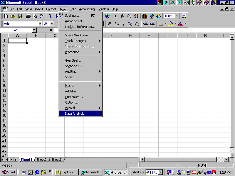
If you have Data Analysis..., then you are all set to use it. If not, we can probably install it fairly easily. Press Tools, then click on "Add-Ins..." A new menu will appear:
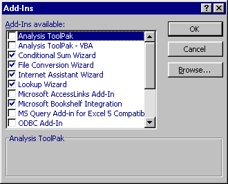
Click on the box next to "Analysis ToolPak" (but leave "Analysis ToolPak - VBA" alone - whether or not it is checked). Clicking on the box next to "Analysis ToolPak" should put a check mark next to "Analysis ToolPak."

Then click on OK. This is probably all that is required to install "Analysis ToolPak." However, in some unusual cases it may ask you to put your Microsoft CD in your computer. If so, do so. Now, when you go back to the Tool menu, you should have Data Analysis...
In the same location you found this file. You should also find files on how to use functions or the Data Analysis tool to calculated various types of statistical solutions. The name of those files describing how to use statistical functions start with "statfun." The name of those files describing how to use the Data Analysis tool start with "DA."
Oh Oh Oh
Oh Oh Oh Oh!! One last thing before you go. Each Excel file is a workbook that usually contains more that one worksheet. Notice that at the bottom of your spreadsheet you see some tabs saying Sheet1, Sheet2, and Sheet3.
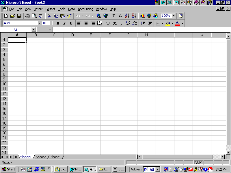
The tab with the white background (Sheet1 in the picture above) is the active worksheet. If you click on another tab (say, Sheet2), that worksheet will become the active worksheet. You can rename the tabs by right clicking on them, selecting "rename" from the menu that appears, then typing in the new name.
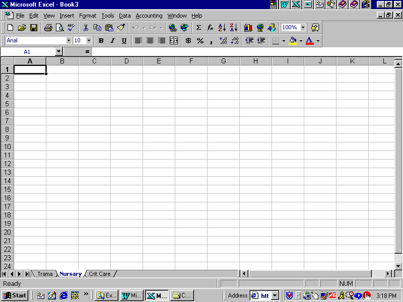
You can insert new spreadsheets using the Insert menu and remove spreadsheets using the Edit menu. Bye, see you later. Of course I can't let you leave without a parting gift. Here is a list of Arithmetic Operators:
|
Arithmetic |
Addition |
Division |
Exponent |
Multiplication |
Percentage |
Subtraction |
|
Example |
=5+6 |
=6/3 |
=2^3 |
=2*3 |
=2% |
=5-4 |
|
Answer |
11 |
2 |
8 |
6 |
.02 |
1 |